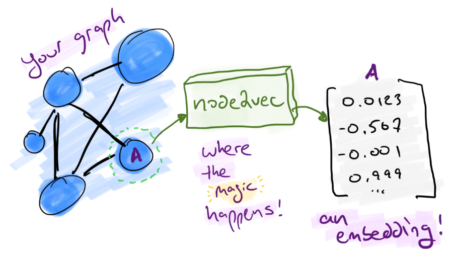
Figure 1: Graph Embeddings are Magical!
Since most machine learning and artificial intelligence applications expect someone to present them just numerical representations of the real world, some non-trivial amount of time is spent turning pictures of cats on the internet into 1’s and 0’s. You can do the same with your graphs, but there’s a catch.
A disclaimer: this post was written using a pre-release of v1.3 of the Graph Data Science library and some of the examples here may need tuning, especially since the node2vec implementation is still in an alpha1 state.
node2what-now? 🤔
As the name implies, node2vec creates node embeddings for the given nodes of a graph, generating a d-dimensional feature vector for each node where d is a tunable parameter in the algorithm.
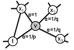
Figure 2: A biased random walk with node2vec (image from the paper)
Ok…so what’s the point and what exactly is a graph embedding?
Embed all the Things
A graph embedding is an expression of the features of a graph in a more traditional format used in data science: feature vectors. Features of a graph can correspond to things like the connectedness (or lack thereof) of a node to others.
Given an arbitrary graph, how can you scalably generate feature vectors? For small graphs, we could make something pretty trivial by hand. But as graphs grow or are have unknown characteristics you’ll need a general approach that can learn features from the graph and do so at scale.
How does node2vec do it?
This is where node2vec comes in. It utilizes a combination of feature learning and a random walk to generalize and scale.
This means node2vec doesn’t:
- need to know specifics of what your graph represents
- really care about the size of the graph
- can be used for embedding arbitrary undirected monopartite graphs
The nitty-gritty is beyond the scope of this blog post, so if you’re of an academic mindset I recommend reading Grover and Leskovec’s paper node2vec: Scalable Feature Learnings for Networks.
The Les Misérables Data Set
Similar to Neo4j’s often demo’d Game of Thrones data set, let’s take look at one used by the node2vec authors related to co-appearances in the Victor Hugo novel Les Misérables.
And just like Game of Thrones, I haven’t read Les Misérables. Shhh!
Using the node2vec paper, let’s see if we can leverage the Neo4j implementation in the GDS library to create something similar to what the author’s published in their case study.
Prerequisites
Grab a copy of Neo4j 4.1, ideally a copy of Neo4j Desktop to make it easier for yourself if you’re not familiar with installing plugins, etc. (See the getting started guide if you’re new to this stuff.)
You’ll need the latest supported APOC and Graph Data Science plugins (v1.3!) as well.
Loading the Data
I’ve transformed a publicly available data set from Donald Knuth’s “The Stanford GraphBase: A Platform for Combinatorial Computing”2 into a JSON representation easily loaded via APOC’s json import procedure.
It doesn’t get much easier than this:
CALL apoc.import.json('https://www.sisu.io/data/lesmis.json')
You should now have a graph with 77 nodes (each with a Character
label) connected to one another via a APPEARED_WITH relationship
containing a weight numerical property.

Figure 3: Initial overview of our Les Mis network
While we’ve loaded it as a directed graph (because all relationships in Neo4j must have a direction), our data set is really representing an undirected graph.
Feel free to explore it a little. One of the interesting things is this data set already contains some modularity-based clustering (since I got the source data from the Gephi project). We’ll use this later to compare/contrast our output.
Using node2vec
Now that we’ve got our undirected, monopartite3 graph how do we use node2vec? Just like other GDS algorithms, we define our graph projection and set some algorithm specific parameters.
In the case of node2vec, the parameters we’ll tune are:
embeddingSize- (integer) The number of dimensions of the resulting feature vector
returnFactor- (double) Likelyhood of returning to the prior node in the random walk (referred to as p in the node2vec paper)
inOutFactor- (double) Bias parameter for how likely the random walk will explore distant nodes vs. closer nodes in the graph (reffered to as q in the node2vec paper)
walkLength- (integer) The length of each random walk
Note: All of the above parameters take non-negative values. 😉
Using parameter placeholders, here’s what a call to node2vec looks like using an anonymous, native graph projection:
CALL gds.alpha.node2vec.stream({
  nodeProjection: 'Character',
  relationshipProjection: {
  EDGE: {
    type: 'APPEARED_WITH',
    orientation: 'UNDIRECTED'
  },
  embeddingSize: $d,
  returnFactor: $p,
  inOutFactor: $q,
  walkLength: $l
}) YIELD nodeId, embedding
Reproducing Grover & Leskovec’s Findings
In their paper, the authors leverage the Les Mis’ data set to illustrate the tunable return (p) and in-out (q) parameters and how they influence the resulting feature vectors and, consequently, the impact to the output of a k-means clustering algorithm. Let’s use Neo4j’s node2vec algorithm and see how we can reproduce Grover & Leskovec’s case study in the Les Mis network4.
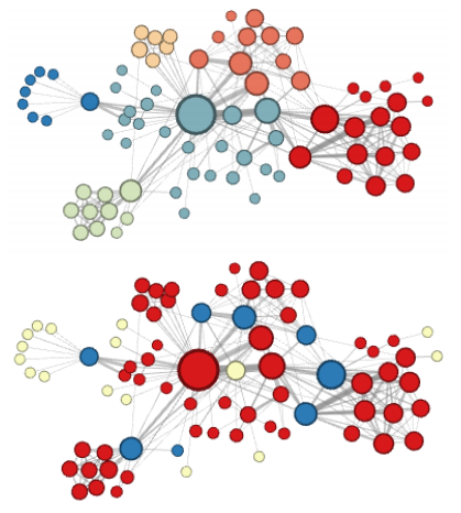
Figure 4: Grover and Leskovec’s “complementary visualizations of Les Mis…” showing homophily (top) and structural equivalence (bottom) where colors represent clusters
What did they demonstrate?
The author’s used the Les Mis network to show how node2vec can discover embeddings that obey the concepts of homophily and structural equivalence. What does that mean?
- homophily
- One definition outside math is “the tendency of individuals to associate with others of the same kind”5. This means favoring nodes in a given node’s neighborhood. (See the top part of fig 4.)
- structural equivalence
- Two nodes are structurally equivalent if they have the same relationships (or lack thereof) to all other nodes6. (See the bottom part of fig 4.)
In terms of Les Mis, homophily can be thought of as clusters of Characters that frequently appear with one another. Basically the traditional idea of “communities.”
For structured equivalence, the example the authors provide is the concept of “bridge characters” that span sub-plots in the Les Mis storyline. These characters might not be part of traditional communities, but act as ways to connect disparate communities. (You might recall in my PaySim 1st-party fraud post the concept of detecting “lyncpins” in a fraud network…sounds sort of similar!)
Let’s see if we can use the parameters they mentioned and a k-means implementation to recreate something similar to their output in Figure 2.
Our Methodology
Since Grover & leskovec don’t mention exactly how they arrived at their Les Mis output, we’re going to try using the following methodology:
- Populate Neo4j with the Co-appearance graph – We’ve already done this part in Loading the Data above!
- Refactor the graph to accomodate unweighted edges – The current alpha node2vec implementation doesn’t support weights yet, but we can achieve the same result through a structural change.
- Generate node embeddings.
- Run the embeddings through scikitlearn’s KMeans algorithm.
- Update the nodes their cluster assignments, writing back to Neo4j.
- Visualize the results with Neo4j Bloom.
Now, let’s get to it!
The Demonstration
We’ve already got the data loaded, so let’s skip to step 2.
Refactoring the Graph
Since the node2vec implementation doesn’t support weighted edges
(yet!), we can achieve the same effect with a simple
refactor. Ultimately, we want the number of co-appearances to be the
weight of the edge between two characters and that’s what the weight
relationship property currently represents.
Since the weight needs to influece the search bias in the node2vec algorithm, we want to increase the probability of a visit to a neighboring node that has a higher weight. How can we do that? Adding multiple edges between nodes!
Let’s take an example:
// Let's look at 2 characters and how they're related
MATCH p=(c1:Character)-[]-(c2:Character)
WHERE c1.name IN ['Zephine', 'Dahlia']
  AND c2.name IN ['Zephine', 'Dahlia']
RETURN p

Figure 5: Zephine and Dahlia (original)
In this case, their APPEARED_WITH relationship has a weight of
4.0. (Not visible in the figure, so trust me!)
What we really want are 4 edges between them, so we can do a little refactoring of our graph:
MATCH (c1:Character)-[r:APPEARED_WITH]->(c2:Character)
UNWIND range(1, r.weight) AS i
  MERGE (c1)-[:UNWEIGHTED_APPEARED_WITH {idx:i}]->(c2)
Now let’s look at Zephone and Dahlia again:

Figure 6: Zephine and Dahlia (now including unweighted edges)
We’ve now got 4 distinct UNWEIGHTED_APPEARED_WITH edges between
them. (Yes, I’m pretty verbose with my naming!)
Generating the Embeddings
This part is made super simple by the GDS library, as we saw above in the using node2vec introduction. We just need to make sure to update the projection and set our parameters.
To start, for the homophily example we set p = 1.0, q = 0.5, d = 16 per Grover & Leskovec’s case study.
CALL gds.alpha.node2vec.stream({
  nodeProjection: 'Character',
  relationshipProjection: {
    EDGE: {
      type: 'UNWEIGHTED_APPEARED_WITH',
      orientation: 'UNDIRECTED'
    }
  },
  returnFactor: 1.0, // parameter 'p'
  inOutFactor: 0.5,  // parameter 'q'
  embeddingSize: 16  // parameter 'd'
})
For our structured equivalence example, the authors set p = 1.0, q = 2.0, d = 16 (in effect, only q changes):
CALL gds.alpha.node2vec.stream({
  nodeProjection: 'Character',
  relationshipProjection: {
    EDGE: {
      type: 'UNWEIGHTED_APPEARED_WITH',
      orientation: 'UNDIRECTED'
    }
  },
  returnFactor: 1.0, // parameter 'p'
  inOutFactor: 2.0,  // parameter 'q'
  embeddingSize: 16  // parameter 'd'
})
What do some of the some of our embeddings results look like? Let’s take a look in Neo4j Browser:
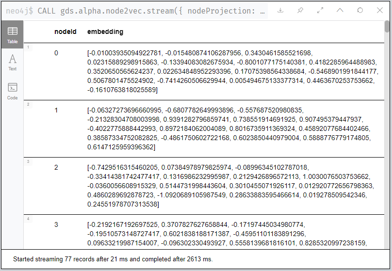
Figure 7: Here, have some node embeddings!
You’ll notice your results differ from mine, regardless of which of
the above examples you run. (If not…I’d be a bit surprised!) Given
the random nature of the walk, the specific values themselves aren’t
interesting or have any reasonable representation. You should see, for
each node, a 16-dimensional feature vector since we set our
dimensions parameter d = 16.
The idea here is the features as a whole describe the nodes with respect to each other. So don’t worry if you can’t make heads or tails of the numbers!
Clustering our Nodes with K-Means
This is where things get a bit fun as you should now be wondering “how do I get the data out of Neo4j and into SciKit Learn?!”
We’re going to use the Neo4j Python Driver to orchestrate running our GDS algorithms and feeding the feature vectors to a k-means algorithm.
Bootstrapping your Python3 environment
In the interest of time, I’ve done the hard part for you. You can git clone my les-miserables project locally and do the following to get going.
-
Create your Python3 Virtual Environment
After cloning or downloading the project, create a new Python virtual environment (this assumes a unix-like shell…adapt for Windows):
$ python3 -venv .venv
-
Activate the environment
$ . .venv/bin/activate
-
Install the dependencies using PIP
$ pip install -r requirements.txtYou should now have
scikit-learnandneo4jpackages available. Feel free to test by opening a Python interpreter and trying toimport neo4j, etc.
Using my provided Python script
I’ve provided an implementation of the Python Neo4j driver as well as
the SciKit Learn KMeans algorithm so we won’t go into details on
eithers inner workings here. The script (kmeans.py)7 takes a variety
of command line arguments allowing us to tune the parameters we
want.
You can look at the usage details using the -h flag:
$ python kmeans.py -h
usage:   kmeans.py [-A BOLT URI default: bolt://localhost:7687] [-U USERNAME (default: neo4j)] [-P PASSWORD (default: password)]
supported parameters:
        -R RELATIONSHIP_TYPE (default: 'UNWEIGHTED_APPEARED_WITH'
        -L NODE_LABEL (default: 'Character'
        -C CLUSTER_PROPERTY (default: 'clusterId'
        -d DIMENSIONS (default: 16)
        -p RETURN PARAMETER (default: 1.0)
        -q IN-OUT PARAMETER (default: 1.0)
        -k K-MEANS NUM_CLUSTERS (default: 6)
        -l WALK_LENGTH (default: 80)
Easy, peasy! (See the appendix for details on the Python implementation.)
The paper mentions what to set p and q to, but what about the
number of clusters? If you count the distinct colors in their visual,
we can see they use the following:
- six clusters for the homophily demonstration
- three clusters for the structural equivalence demonstration
So we’ll set k accordingly.
Do one run for the homophily output and one for the structured
equivalence case (adust the bolt, username, and password params as
needed for your environment) using our parameters for p, q, and
k:
$ python kmeans.py -p 1.0 -q 0.5 -k 6 -C homophilyCluster
Connecting to uri: bolt://localhost:7687
Generating graph embeddings (p=1.0, q=0.5, d=16, l=80, label=Character, relType=UNWEIGHTED_APPEARED_WITH)
...generated 77 embeddings
Performing K-Means clustering (k=6, clusterProp='homophilyCluster')
...clustering completed.
Updating graph...
...update complete: {'properties_set': 77}
And another run changing q = 2.0 to bias towards structured
equivalence and k = 3:
$ python kmeans.py -p 1.0 -q 2.0 -k 3 -C structuredEquivCluster
Connecting to uri: bolt://192.168.1.167:7687
Generating graph embeddings (p=1.0, q=0.5, d=16, l=80, label=Character, relType=UNWEIGHTED_APPEARED_WITH)
...generated 77 embeddings
Performing K-Means clustering (k=6, clusterProp='structuredEquivCluster')
...clustering completed.
Updating graph...
...update complete: {'properties_set': 77}
⚠ HEADS UP! Make sure you use the same cluster output properties (
-Csettings) so they line up with the Bloom perspective I provide!
Nice…but how should we visualize the output?
Visualizing with Neo4j Bloom
If you took my advice and used Neo4j Desktop, you’ll have a copy of Neo4j Bloom available for free. If not, you’re on your own here and you’ll have to just follow along. (Sorry…not sorry.)
Configuring our Perspective
Bloom relies on “perspectives” to tailor the visual experience of the
graph. I’ve done the work for you (you’re welcome!) and you can
download the json file here or find LesMis-perspective.json in the
GitHub project you cloned earlier.
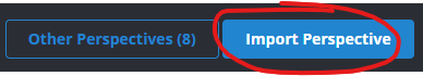
Figure 8: Click the Import button…it’s pretty easy!
Follow the documentation on installing/importing a perspective if you need help.
Visualize the graph
Let’s pull back a view of all the Characters and use the original
APPEARED_WITH relationship type to connect them.
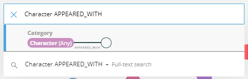
Figure 9: Query for Characters that have a APPEARED_WITH relationship
You should get something looking like the following:
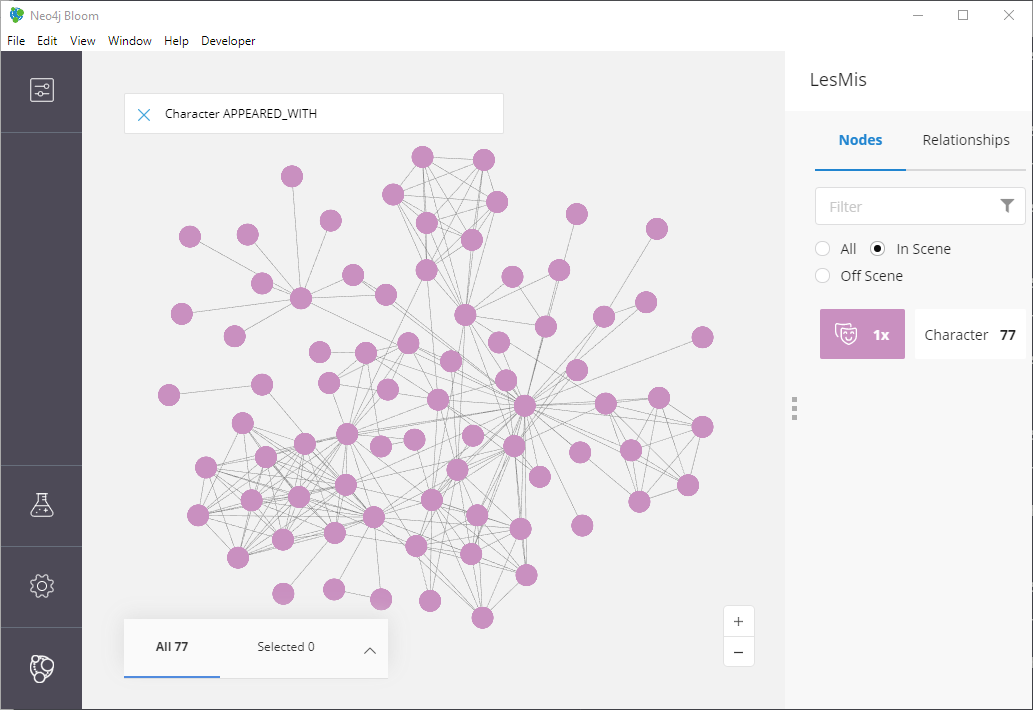
Figure 10: The LesMis Network
There aren’t any colorful clusters and things look pretty messy to me! Let’s toggle the conditional styling to show the output of our clustering.
Using the Bloom node style pop-up menus, you can toggle the perspective’s pre-set rule-based styles:
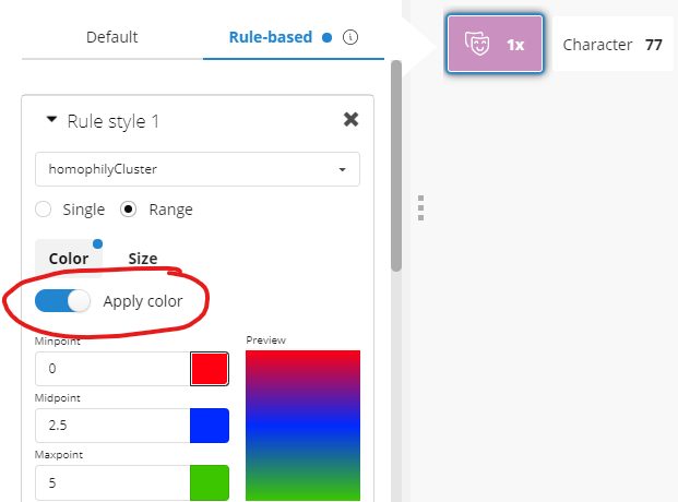
Figure 11: Toggling conditional styling in Bloom
You should now have a much more colorful graph to look at and let’s dig into what we’re seeing.
Our Homophily Results
What should you be seeing at this point? Since we generated embeddings that leaned towards expressing homophily, we should see some obvious communities assigned distinct colors based on the k-means clustering output.
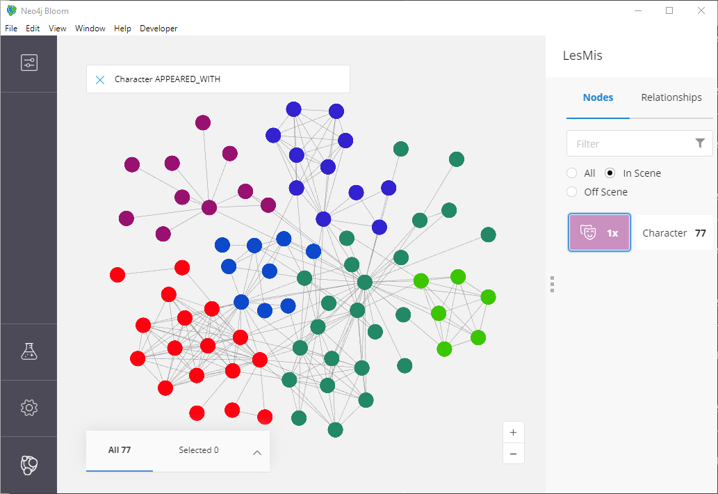
Figure 12: Our homophily results: some nice little clusters!
Not bad! Looks similar to the top part of our screenshot from the node2vec paper.
How about the structural equivalence results?
Our Stuctural Equivalence Results
Oh…oh no. This looks nothing like what is in the node2vec paper!
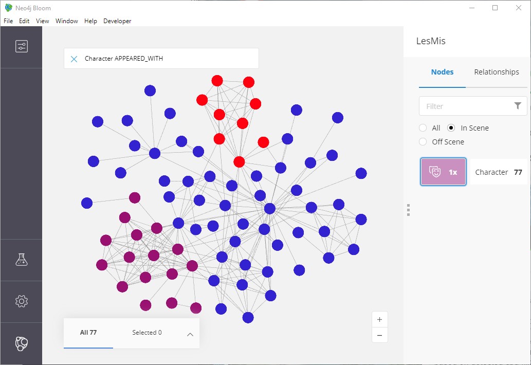
Figure 13: Structural Equivalance results that are…less than ideal!!
What went wrong?! We expected to see something that doesn’t look like typical communities and instead showing the idea of “bridge characters” (recall from our previous definitions of structural equivalence).
Remember our Walk Length parameter?
Earlier I mentioned that the Les Mis network has only 77 nodes. It’s extremely small by any means. Can you remember what the current default walk length parameter is for the node2vec implementation?
Here’s a hint: it defaults to
80😉
That’s fine for our homophily example as the idea was to account for global structure of the graph and build communities. But for finding “bridge characters”, we really care about local structure. (A bridge character bridges close-by clusters and sits between them so should have little to no relation to a “far away” cluster.)
Let’s re-run with a new walk length
So what should we use? Well, I did some testing, and found that l = 7 is a pretty good setting. It’s “local enough” to capture bridging
structure without biasing towards global clusters.
Using the script, add the -l command line argument like so:
$ python kmeans.py -p 1.0 -q 2.0 -k 3 -C structuredEquivCluster -R UNWEIGHTED_APPEARED_WITH -l 7
Here’s what it looks like now:
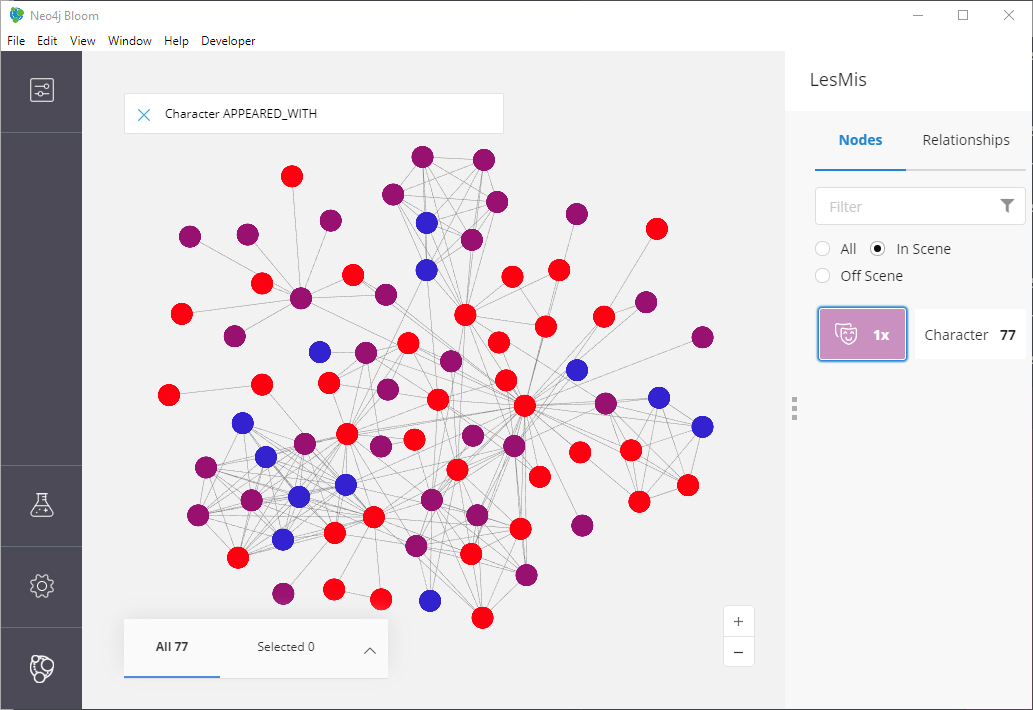
Figure 14: Structural Equivalance, for real this time.
That’s much, much more like the original findings from the paper!
If you count, we get our expected 3 different colors (since in this
case we set k = 3) and if we look at the blue nodes they tend to
connect the reds and purple-ish colored nodes. It’s not a perfect
reproduction of the paper’s image, but keep in mind the authors never
shared their exact parameters!
Note: since we’re using such a small network in these examples, you might have some volatility in your results using a short walk length. That’s ok! Remember it’s a random walk. In practice you’d most likely use a much larger (i.e. well more than 77 nodes) graph and locality would be more definable.
Where can we go from here?
Depending on your interests, I recommend two different next steps if you’d like to learn more (beyond just continuing to use node2vec).
Operationalizing your Graph Data Science
One area worth exploring is how to better integrate Neo4j into your existing ML workflows and pipelines. In the above example, we just used the Python driver and anonymous projections to integrate something pretty trivial…but you probably need to handle much larger data sets in your use cases.
One possibility is leveraging Neo4j’s Apache Kafka integration in the neo4j-streams plugin. Neo4j’s Ljubica Lazarevic provides an overview in her January 2019 post: How to embrace event-driven graph analytics using Neo4j and Apache Kafka
GraphSAGE
Another area to explore might be a different graph embedding algorithm: GraphSAGE8
An implementation of GraphSAGE is also available as part of the new GDS v1.3 (in alpha form) and takes a different approach from node2vec.
Appendix: Neo4j’s Python Driver and SciKit Learn
Here are some code snippets that help show what’s going on under the
covers in the kmeans.py script. A lot of the code is purely
administrative (dealing with command line args, etc.), but there are
two key functions.
Extracting the Embeddings
How do you run the GDS node2vec procedure and get the embedding
vectors? This is one way to do it, but the key part is using
session.run() and adding in the query parameters.
def extract_embeddings(driver, label=DEFAULT_LABEL, relType=DEFAULT_REL,
                       p=DEFAULT_P, q=DEFAULT_Q, d=DEFAULT_D, l=DEFAULT_WALK):
    """
    Call the GDS neo2vec routine using the given driver and provided params.
    """
    print("Generating graph embeddings (p={}, q={}, d={}, l={}, label={}, relType={})"
          .format(p, q, d, l, label, relType))
    embeddings = []
    with driver.session() as session:
        results = session.run(NODE2VEC_CYPHER, L=label, R=relType,
                              p=float(p), q=float(q), d=int(d), l=int(l))
        for result in results:
            embeddings.append(result)
    print("...generated {} embeddings".format(len(embeddings)))
    return embeddings
Where NODE2VEC_CYPHER is our Cypher template:
NODE2VEC_CYPHER = """
CALL gds.alpha.node2vec.stream({
  nodeProjection: $L,
  relationshipProjection: {
    EDGE: {
      type: $R,
      orientation: 'UNDIRECTED'
    }
  },
  embeddingSize: $d,
  returnFactor: $p,
  inOutFactor: $q
}) YIELD nodeId, embedding
"""
Clustering with SciKit Learn
Our above function returns a List of Python dicts, each with a
nodeId and embedding key where the embedding is the feature
vector (as a Python List of numbers).
To use SciKit Learn, we need to generate a dataframe using NumPy,
specifically the array() function. Using a list comphrension, it’s
easy to extract out just the feature vectors from the
extract_embedding output:
def kmeans(embeddings, k=DEFAULT_K, clusterProp=DEFAULT_PROP):
    """
    Given a list of dicts like {"nodeId" 1, "embedding": [1.0, 0.1, ...]},
    generate a list of dicts like {"nodeId": 1, "valueMap": {"clusterId": 2}}
    """
    print("Performing K-Means clustering (k={}, clusterProp='{}')"
          .format(k, clusterProp))
    X = np.array([e["embedding"] for e in embeddings])
    kmeans = KMeans(n_clusters=int(k)).fit(X)
    results = []
    for idx, cluster in enumerate(kmeans.predict(X)):
        results.append({ "nodeId": embeddings[idx]["nodeId"],
                         "valueMap": { clusterProp: int(cluster) }})
    print("...clustering completed.")
    return results
The last part, after using KMeans, is constructing a useful output
for populating another Cypher query template. My approach creates a
List of dicts that like:
[
    { "nodeId": 123, "valueMap": { homophilyCluster: 3 } },
    { "nodeId": 234, "valueMap": { homophilyCluster: 5 } },
    ...
]
Which drives the super simple, 3-line bulk-update Cypher template:
UPDATE_CYPHER = """
UNWIND $updates AS updateMap
    MATCH (n) WHERE id(n) = updateMap.nodeId
    SET n += updateMap.valueMap
"""
Using Cypher’s UNWIND, we iterate over all the dicts. The MATCH
finds a node using the internal node id (using id()) and then
updates properties on the matched node using the += operator and the
valueMap dict.
-
What’s alpha state mean? See the GDS documentation on the different algorithm support tiers: https://neo4j.com/docs/graph-data-science/current/algorithms/ ↩︎
-
D. E. Knuth. (1993). The Stanford GraphBase: A Platform for Combinatorial Computing, Addison-Wesley, Reading, MA ↩︎
-
Monopartite graphs are graphs where all nodes share the same label or type…or lack labels. ↩︎
-
See section 4.1 Case Study: Les Misérables network in the node2vec paper ↩︎
-
See http://faculty.ucr.edu/~hanneman/nettext/C12%5FEquivalence.html#structural ↩︎
-
Source code is also here: https://github.com/neo4j-field/les-miserables/blob/master/kmeans.py ↩︎