If you’ve followed along in the PaySim series of posts or at least discovered the demo project, you’ve now got a graph representing 30 days of financial transactions in a simulated financial network running inside your Neo4j 3.5 database.
Somewhere in that haystack are our fraudsters we created previously, or at least the result of their malicious behavior.
The question is: How can we leverage the fact we’ve built a graph to rapidly identify potential first party fraudsters?
Looking for previous posts? See part 1 to learn about PaySim and part 2 to learn about integrating it with Neo4j.
For instructions on installing Neo4j’s Graph Data Science library, see the documentation here.
What’s our Graph look like again?
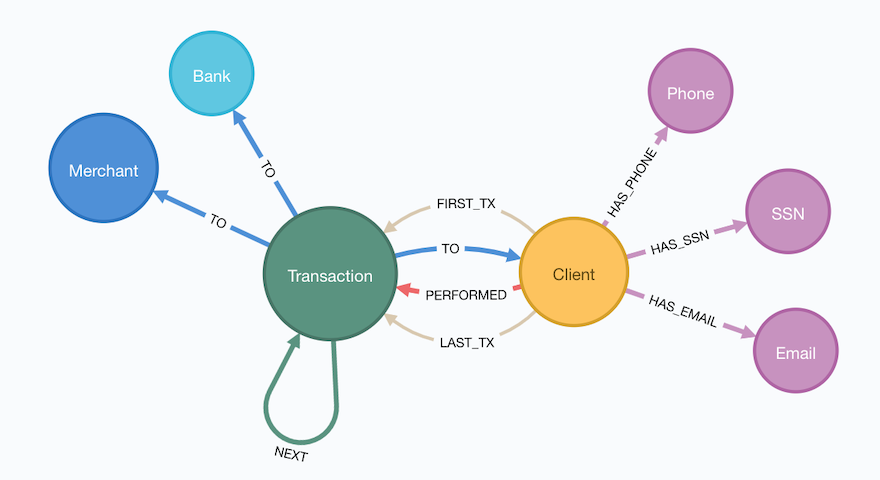
Before we dig into our methodology and look at some queries, let’s first recap and look at the graph we built and loaded in Part 2.
Now that’s just the schema of our graph, but what are defining characteristics of our data? We can use a mix of Cypher and helper procedures from APOC to profile our graph.
CALL db.labels() YIELD label
CALL apoc.cypher.run('MATCH (:`'+label+'`) RETURN count(*) as freq',{}) YIELD value
WITH label,value.freq AS freq
CALL apoc.meta.stats() YIELD nodeCount
WITH *, 10^3 AS scaleFactor, toFloat(freq)/toFloat(nodeCount) AS relFreq
RETURN label AS nodeLabel,
    freq AS frequency,
    round(relFreq*scaleFactor)/scaleFactor AS relativeFrequency
ORDER BY freq DESC
The above Cypher will:
- interrogate the database to get all known labels (e.g. Client, Transaction, etc.)
- Run a sub-query using APOC to get label counts
- Analyze the label counts against the global label counts
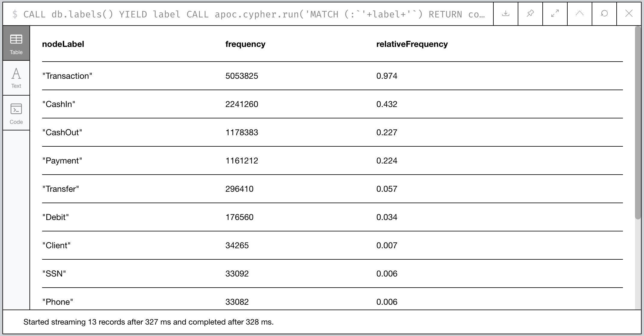
Figure 1: Relative Frequency of Labels in our PaySim Graph
So most (62%) of our transaction activity is some form of
ingress/egress where money flows into and out of the network via
CashIn=/=CashOut transactions. The remaining 38% of activity
involves money flowing to and from parties in the network.
Is there anything interesting about the transactions themselves?
Let’s take a look.
// Get the total number of transactions in count, value, and frequency
MATCH (t:Transaction)
WITH sum(t.amount) AS globalSum, count(t) AS globalCnt
WITH *, 10^3 AS scaleFactor
UNWIND ['CashIn', 'CashOut', 'Payment', 'Debit', 'Transfer'] AS txType
    CALL apoc.cypher.run('MATCH (t:' + txType + ') RETURN sum(t.amount) as txAmount, count(t) AS txCnt', {}) YIELD value
    RETURN txType,
        value.txAmount AS TotalMarketValue,
        100 * round(scaleFactor * (toFloat(value.txAmount) / toFloat(globalSum)))/scaleFactor AS `%MarketValue`,
        100 * round(scaleFactor * (toFloat(value.txCnt) / toFloat(globalCnt)))/scaleFactor AS `%MarketTransactions`,
        toInteger(toFloat(value.txAmount) / toFloat(value.txCnt)) AS AvgTransactionValue,
        value.txCnt AS NumberOfTransactions
    ORDER BY `%MarketTransactions` DESC
The above Cypher performs a pretty basic aggregation of the number of transactions by type, the total monetary value, and the average value of each transaction.
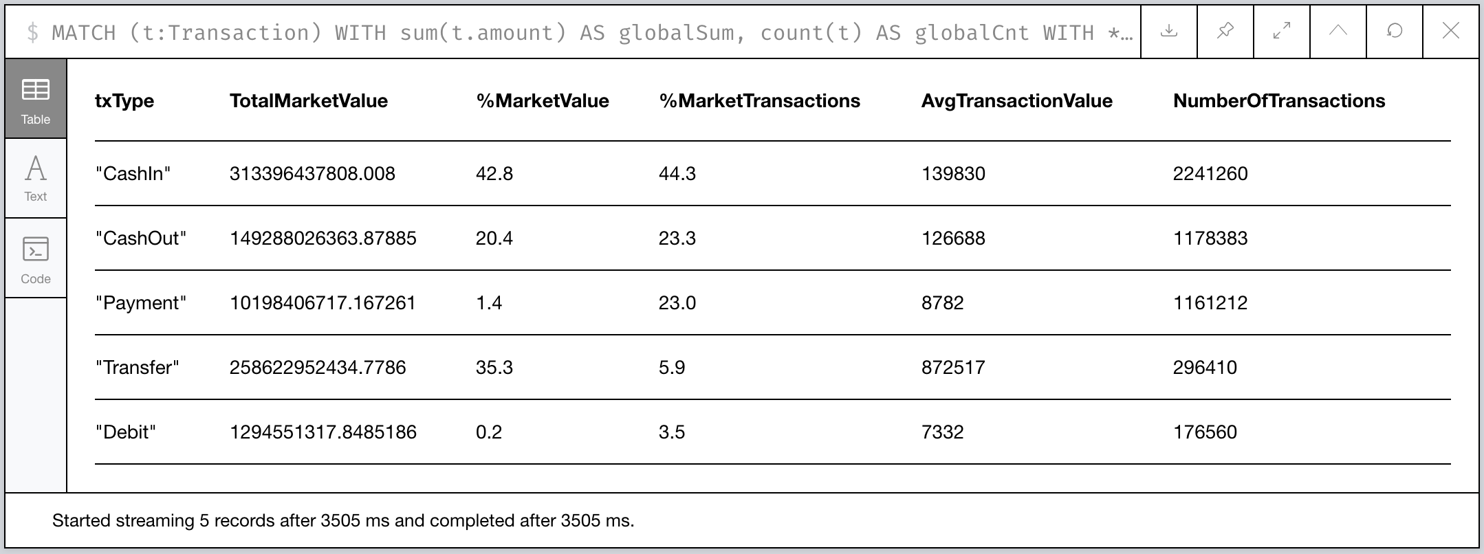
Figure 2: Aggregate Transaction statistical profile
The CashIn transactions still dominate in terms of quantity and
average transaction size, but interestingly Transfer transactions
make up over a 1/3rd of the total market activity in terms the amount
of money involved even though they’re hardly 6% of the total
transaction volume. In fact, the average Transfer involves funds
6.25 times the average CashIn transaction!!
What does this mean? 🧐
Money is passed around in large quantities more than its injected into or removed from the network.1
Given that fact, we’ll probably see something interesting when we look at transfers of money between Clients!
Finding our First Party Fraud
Recall that First Party Fraud is a form of identity fraud where the fraudster either uses either fully synthetic (fake) identifiers or steals and uses real identifiers in order to build up some account standing (e.g. credit rating or credit line) before “busting out” and draining the account into something liquid they can run away with.
In our PaySim version, we’ve constructed 1st Party Fraudsters that
generate pools of identifiers like Emails, SSNs, and Phone
Numbers that they remix into different (ideally unique) combinations
when creating a client in our network. Then at some time in the
future, they drain those accounts via an intermediary (a mule) and
conduct a CashOut to exfiltrate the money from our network.
Our methodology for finding these fraudulent accounts will be as follows:
- Cull the universe down to potentially fruadulent accounts using community detect methods.
- Quantify and filter community members based on similarity.
- Identify hot spots (possible initial sources of fraud) using centralitiy measurements.
- Visualize the subgraph to illustrate the impact and any anomalies.
Filtering the Universe with Weakly Connected Components
Our first step leverages the connectedness of our graph and looks for PaySim Clients that share identifiers. Since when we loaded our data in part 2 creating unique nodes for each instance of an identifier (e.g. there’s only one SSN of 123-45-6789), it’s almost trivial to find Clients that share identifiers.
The Weakly Connected Components algorithm analyzes the graph and identifies “graph components”. A component is a set of nodes and relationships where you can reach each member (node) from any other through traversal. It’s called “weakly” since we don’t account for the directionality of relationships.
Connected component algorithms are a type of community detection algorithm. They’re great for understanding the structure of a graph.

Figure 3: “A graph with three components” by David Eppstein (Public Domain, Wikipedia, 2007)
The net result: the algorithm identifies all the possible subgraphs of Clients that have some identifiers in common.
Sounds almost too easy, right? In practice, it’s not uncommon for identifiers to be shared among accounts. A simple example is a shared mailing address for roommates or family members. In real world fraud detection methologies, identifiers tend to be weighted differently.
Create our WCC Projection
Since we don’t care about all nodes and relationships for our WCC approach, we can keep our algorithm focused on just a subgraph and load it into memory.2
Recall our data model we built out in part 1:
Figure 4: The PaySim 2.1 Data Model
In our case, we’re concerned about only 4 label types:
- Client which is our account/account holder
- SSN which is like a US social security number (or Canadian SNI, etc.)
- Email which should be an email address
- Phone which represents someone’s contact phone number
And we only need the relationships that connect nodes of the above labels: HAS_SSN, HAS_EMAIL, HAS_PHONE.
So let’s target the following subgraph:
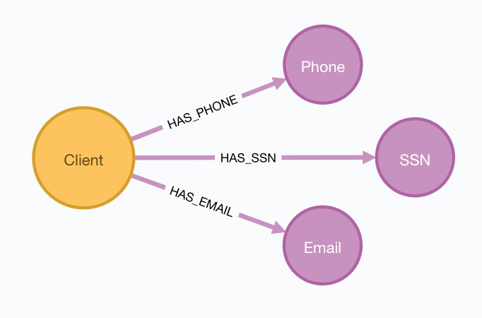
Figure 5: Just our Identifiers in PaySim 2.1
We’ll use the gds.graph.create3 stored procedure and lists of Labels
and Relationships of the part of the graph we want to analyze.
First, let’s estimate how much memory our projection will consume.
CALL gds.graph.create.estimate(
    ['Client', 'SSN', 'Email', 'Phone'],
    ['HAS_SSN', 'HAS_EMAIL', 'HAS_PHONE'])
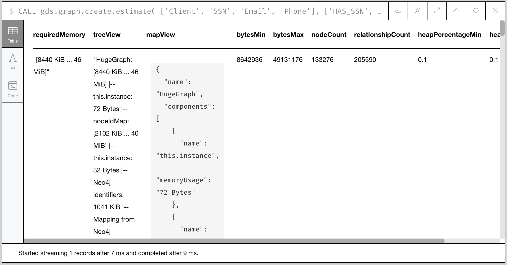
Figure 6: Our estimate for our Graph Projection
According to the requiredMemory output, it looks like we’ll need
about 8-46 megabytes…pretty small! Why is that? We’re focusing only
on Clients and their identifiers, which comprise only ~1-2% of our
total database in terms of nodes. (Recall we analyzed that earlier in
this post.)
Ok, let’s create the projection now. You’ll notice the stored procedure call is similar, but now we also give it a name we’ll use to refer to the projection later:
// Create our projection called "wccGroups"
CALL gds.graph.create('wccGroups',
    ['Client', 'SSN', 'Email', 'Phone'],
    ['HAS_SSN', 'HAS_EMAIL', 'HAS_PHONE'])
You should see some metadata output telling you some details about the type and size of the graph projection. It’ll detail how many relationships and nodes were processed plus some other facts.

Figure 7: Our “wccGroups” graph projection output
Easy, peasy! Let’s get on with running the algorithm…
Compute and tag our WCC groups
With the subgraph loaded, we can simply let the algorithm do its thing. In the interest of learning and sanity checking our work, let’s first look at the algorithm output before we go much further.
The algorithm is accessed via the gds.wcc.stream stored procedure
call and it provides as output the internal id of a given node
(nodeId) and the component it’s a part of (componentId). We’ll use
the utility function gds.util.asNode() to fetch the underlying Node
instance by its internal id and then analyze our groupings:
// Call the WCC algorithm using our native graph projection
CALL gds.wcc.stream('wccGroups') YIELD nodeId, componentId

// Fetch the Node instance from the db and use its PaySim id
WITH componentId, collect(gds.util.asNode(nodeId).id) AS clients

// Identify groups where there are at least 2 clients
WITH *, size(clients) as groupSize WHERE groupSize > 1
RETURN * ORDER BY groupSize DESC LIMIT 1000
Scanning the results, we have a few large clusters and a lot of small clusters. Those large clusters will probably be of interest and we’ll come back to that shortly.
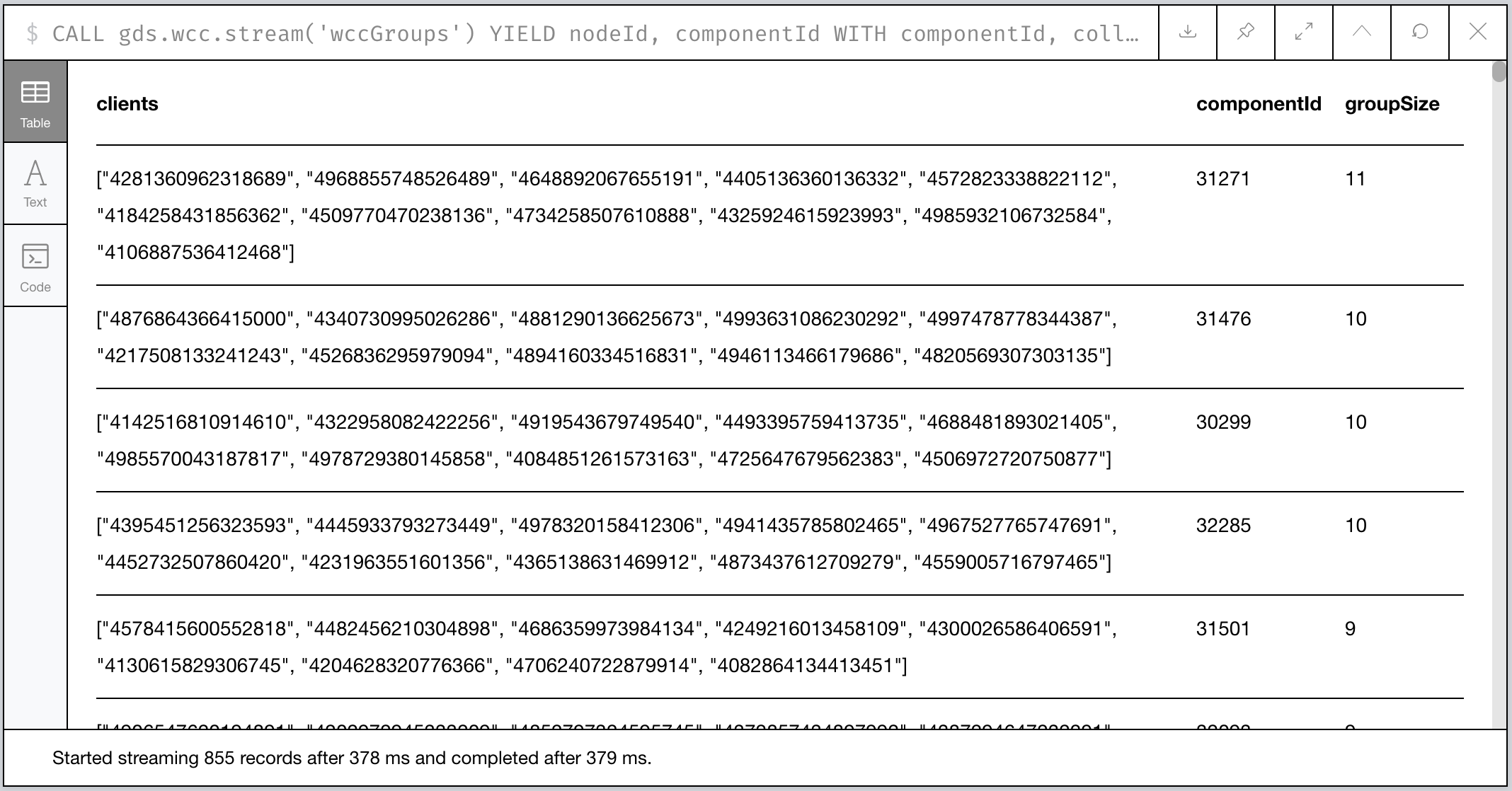
Figure 8: Our largest graph Components per WCC
Now let’s re-run the algorithm and tag our groups!
We’ll give each matching Client node a new property we’ll call
fraud_group and assign the componentId generated by the
algorithm. This will let us recall the groups at will via basic Cypher
against the core database.
// Call the WCC algorithm using our native graph projection
CALL gds.wcc.stream('wccGroups') YIELD nodeId, componentId

// Fetch the Node instance from the db and use its PaySim id
WITH componentId, collect(gds.util.asNode(nodeId).id) AS clientIds
WITH *, size(clientIds) AS groupSize WHERE groupSize > 1

// Note that in this case, clients is a list of paysim ids.
// Let's unwind the list, MATCH, and tag them individually.
UNWIND clientIds AS clientId
    MATCH (c:Client {id:clientId})
    SET c.fraud_group = componentId
For good measure, you should index the fraud_group property for
faster recall. Let’s do that.
CREATE INDEX ON :Client(fraud_group)
Sanity Checking WCC’s Output
Lastly, let’s sanity check our results. A few queries ago we only
glanced at the output, but now that we have groups tagged in our
database and the fraud_group property indexed, let’s take a deeper
look at how the communities shake out.
// MATCH only our tagged Clients and group them by group size
MATCH (c:Client) WHERE c.fraud_group IS NOT NULL
WITH c.fraud_group AS groupId, collect(c.id) AS members
WITH groupId, size(members) AS groupSize
WITH collect(groupId) AS groupsOfSize, groupSize

RETURN groupSize,
        size(groupsOfSize) AS numOfGroups
ORDER BY groupSize DESC
What’s the data look like?
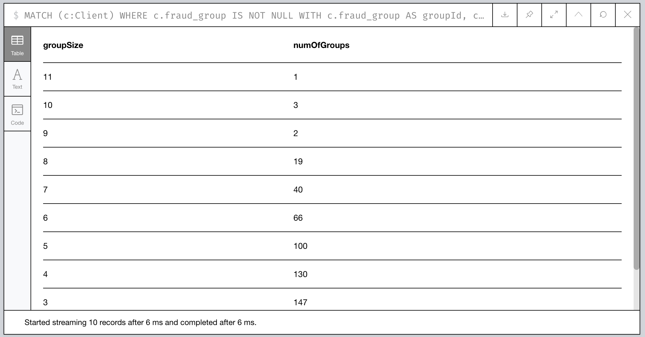
Figure 9: Histogram of Group Size
Ok, wow. Seems most of the communities are pretty small with only 2-3 members, but we have some clear anomalies where 6 groups have community sizes of 9 or more. Something fishy has to be going on with them!
Let’s take a look at them…
// Visualize the larger likely-fraudulent groups
MATCH (c:Client) WHERE c.fraud_group IS NOT NULL
WITH c.fraud_group AS groupId, collect(c.id) AS members
WITH *, size(members) AS groupSize WHERE groupSize > 8

MATCH p=(c:Client {fraud_group:groupId})-[:HAS_SSN|HAS_EMAIL|HAS_PHONE]->()
RETURN p

Figure 10: Our Fraud Groups (of size > 8)
Our six graph components contain a handful of Clients (nodes in yellow) that appear to share identifiers like SSN, Email, and Phone numbers (the nodes in the purplish color).
Analyzing our Suspicious Groups
Now that we’ve identified Client members of some suspicious groups, what if we look at the other Clients outside the group they’ve transacted with?
Maybe we can find something about the true extent of these fraud networks!
Looking at who interacts with our Fraud Groups
Let’s use a simple cypher query to figure out who our fraud groups interact with, maybe there’s something we can learn.
// Recall our tagged Clients and group them by group size
MATCH (c:Client) WHERE c.fraud_group IS NOT NULL
WITH c.fraud_group AS groupId, collect(c.id) AS members
WITH groupId, size(members) AS groupSize WHERE groupSize > 8

// Expand our search to Clients one Transaction away
MATCH p=(:Client {fraud_group:groupId})-[]-(:Transaction)-[]-(c:Client)
WHERE c.fraud_group IS NULL
RETURN p

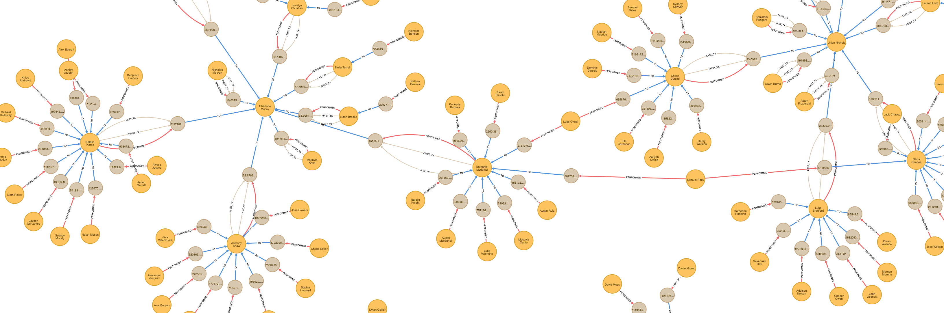
Figure 11: External Transactions with our Large Fraud Groups
Now that’s something…it looks like what we thought were 6 distinct groups might actually be less. One in particular (at the top of the visualization) seems to be a very expansive network with numerous Clients involved.
Let’s do some quick analysis and see what types of Transactions occur between these Clients. With a slight tweak to the query, we can perform some aggregate reporting:
// Recall our tagged Clients and group them by group size
MATCH (c:Client) WHERE c.fraud_group IS NOT NULL
WITH c.fraud_group AS groupId, collect(c.id) AS members
WITH groupId, size(members) AS groupSize WHERE groupSize > 8

// Build our network as before
MATCH (:Client {fraud_group:groupId})-[]-(txn:Transaction)-[]-(c:Client)
WHERE c.fraud_group IS NULL

// Since our PaySim demo stacks labels, let's look at our txn reference
UNWIND labels(txn) AS txnType
    RETURN distinct(txnType), count(txnType)
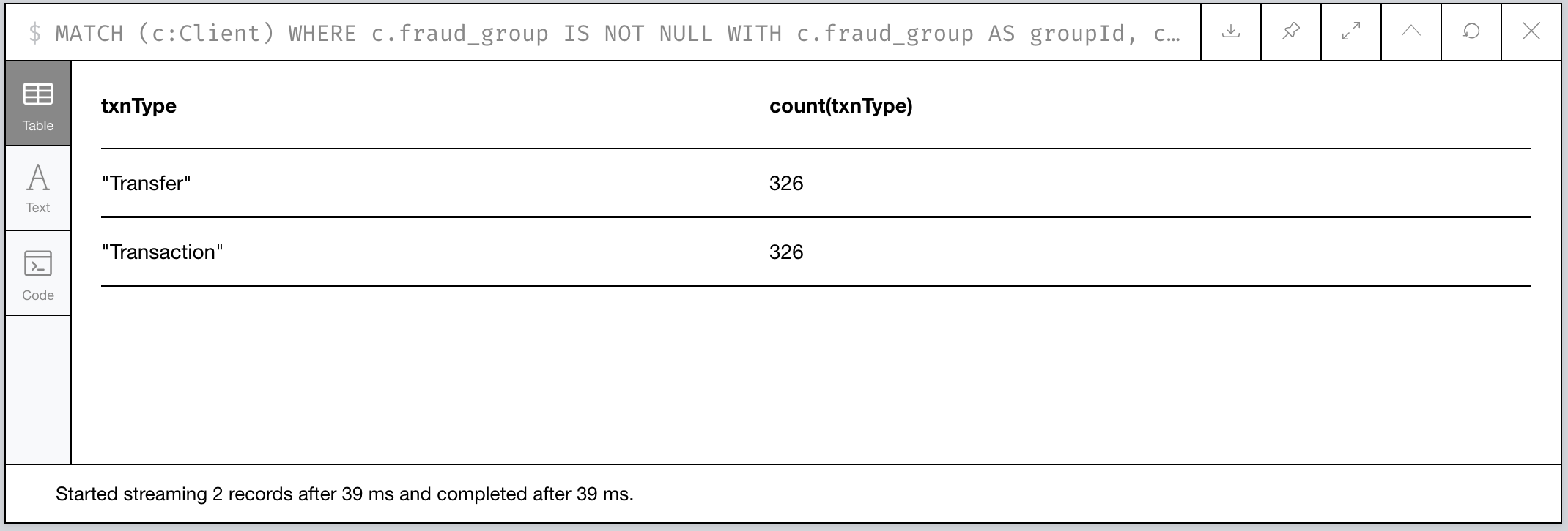
Figure 12: An Analysis of Transactions between our Fraud Groups and Others
WOW! All the transactions that connect other Clients to our fraud groups are all Transfers. Kinda fishy!
Connecting our new 2nd-level Fraud groups
We’ve now identified four potential fraud rings. Let’s tag them and relate them to one another to make further analysis easier.
We’ll simplify how our suspect Clients relate to one another
connecting them via direct TRANSACTED_WITH relationships if they’ve
performed a Transaction with one another:
// Recall our tagged Clients and group them by group size
MATCH (c:Client) WHERE c.fraud_group IS NOT NULL
WITH c.fraud_group AS groupId, collect(c.id) AS members
WITH groupId, size(members) AS groupSize WHERE groupSize > 8

// Expand our search to Clients one Transaction away
MATCH (c1:Client {fraud_group:groupId})-[]-(t:Transaction)-[]-(c2:Client)
WHERE c2.fraud_group IS NULL

// Set these Clients as suspects for easier recall
SET c1.suspect = true, c2.suspect = true

// Merge a relationship directly between Clients and copy some
// of the Transaction properties over in case we need them.
MERGE (c1)-[r:TRANSACTED_WITH]->(c2)
ON CREATE SET r += t
RETURN count(r)
Note: We’ll ignore trying to preserve the directionality of the original Transaction. That’s a lesson left to the reader. 😉
Now how do our simplified 2nd-level groups look?

Figure 13: Our 2nd-Level Fraud Groups
WCC Redux: Quickly identify our new Groupings
We’ll use the WCC algorithm again to tag members of each of the groups, but unlike before we’ll use what’s called a cypher projection4 to define how we’ll target a subgraph.
Plus, since this is a pretty small projection (only a few hundred
nodes), we’ll forego creating a named projection and just run it on
the fly! This time we’ll use the gds.wcc.write procedure that will
run the WCC algorithm and tag our members for us, making this pretty
trivial.
You may wonder, why didn’t we use this procedure before instead of the
gds.wcc.streamprocedure? Well, last time we didn’t want to deal with components with only a single Client because they’re not very suspicicous in our case.
Run the following:
// We now use Cypher to target our Nodes and Relationships for input.
// Note how for relationships, the algorithm just wants to know which
// node relates to another and doesn't actually care about the type!
CALL gds.wcc.write({
    writeProperty: 'fraud_group_2',
    nodeQuery: 'MATCH (c:Client {suspect:true}) RETURN id(c) AS id',
    relationshipQuery: 'MATCH (c1:Client {suspect:true})-[r:TRANSACTED_WITH]->(c2:Client)
                        RETURN id(c1) AS source, id(c2) as target'
})
And like before, we’ll index our new property for faster retrieval:
CREATE INDEX ON :Client(fraud_group_2)
Now let’s analyze our new groups and their memberships:
// Recall our tagged Clients and group them by group size
MATCH (c:Client) WHERE c.fraud_group_2 IS NOT NULL
WITH c.fraud_group_2 AS secondGroupId, collect(c.id) AS members

RETURN secondGroupId, size(members) AS groupSize
ORDER BY groupSize DESC
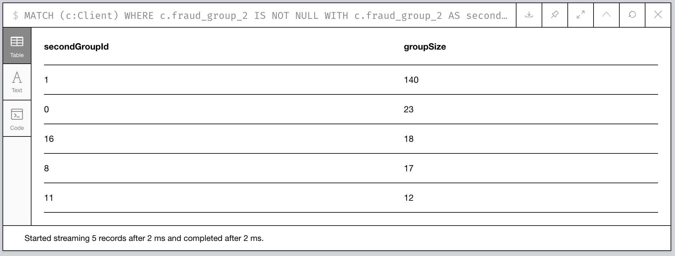
Figure 14: How large are our 2nd Level Fraud Groups?
It looks like the second-level group with id 1 is MASSIVE compared
to the others! Probably a high-value fraud ring we can try breaking up.
Quantitatively Identifying Suspects
First thing we can do is use our eyeballs and our intuition. Graphs make it easy for humans to start asking questions because we’re glorified pattern recognition biocomputers doing it since birth using any of our senses as input.
But how can we do this algorithmically?
Who are our likely Suspects?
Let’s say we want to tackle that massive 140 Client potential fraud ring. Looking at the graph visually, there appear to be 3 Client accounts that tie the whole thing together:
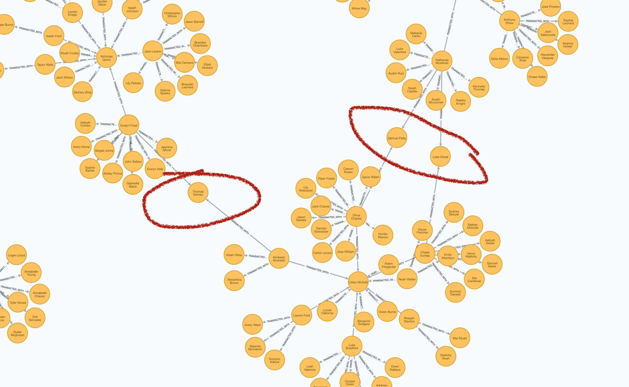
Figure 15: Our potential Targets
How can we programmatically target Thomas Gomez, Samuel Petty, and
Luke Oneal?
Computing Betweenness Centrality
Another algorithm we can leverage is called Betweenness Centrality.5 From the documentation:
Betweenness centrality is a way of detecting the amount of influence a node has over the flow of information in a graph. It is often used to find nodes that serve as a bridge from one part of a graph to another.
Sounds like a great fit! Let’s try it out.
// Target just our largest fraud group (group 1) using a Cypher projection
CALL gds.alpha.betweenness.stream({
        nodeQuery: 'MATCH (c:Client {fraud_group_2:1}) RETURN id(c) AS id',
    relationshipQuery: 'MATCH (c1:Client)-[:TRANSACTED_WITH]-(c2:Client)
                        RETURN id(c1) AS source, id(c2) AS target'
}) YIELD nodeId, centrality

// Fetch the node and also filter out nodes with scores of 0
WITH gds.util.asNode(nodeId) AS c, centrality WHERE centrality > 0

// Return the name and order by score
RETURN c.name AS name, centrality ORDER BY centrality DESC
Let’s take a look at the highest scores:
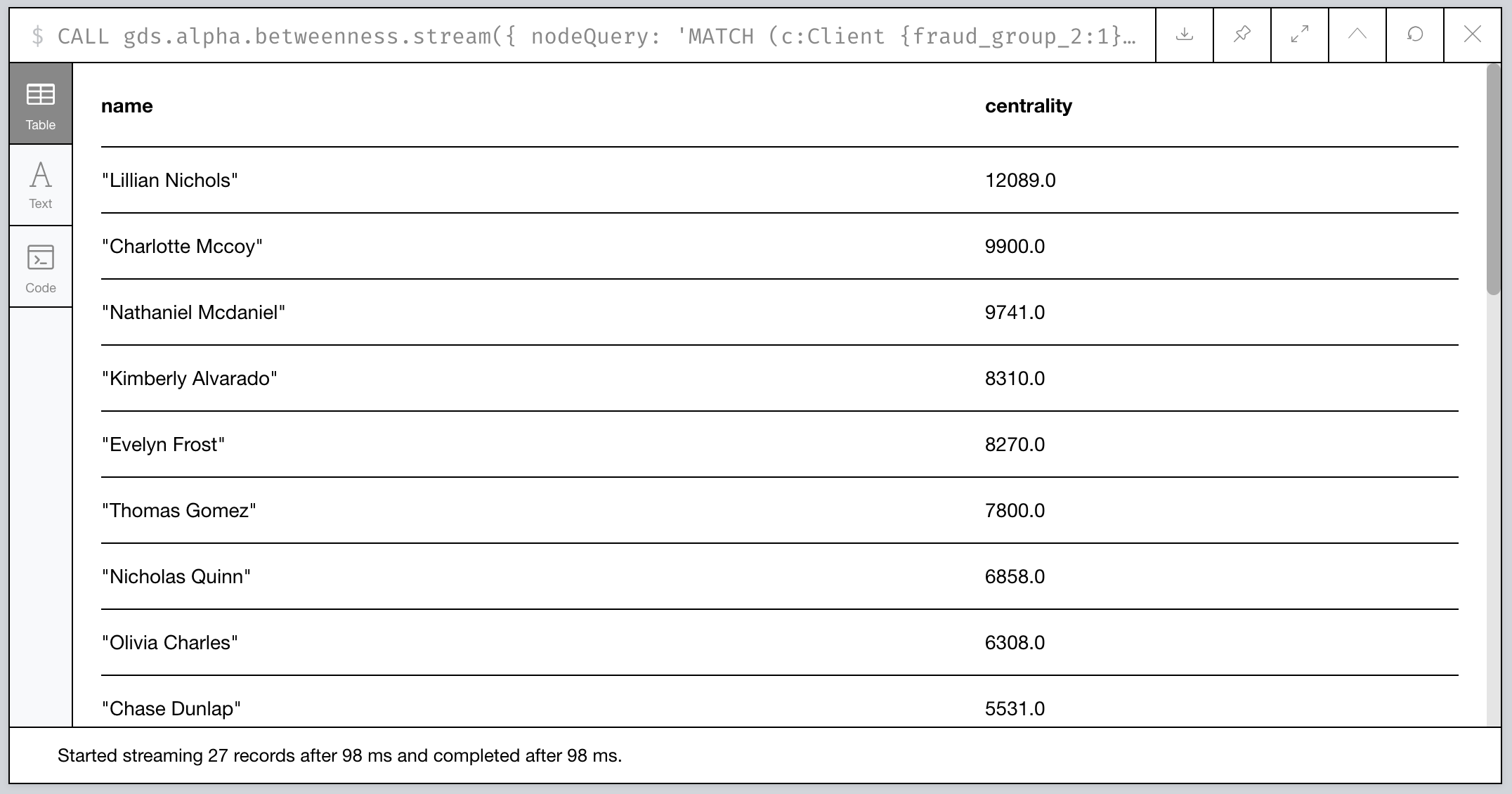
Figure 16: Clients of 2nd Level Fraud Group 1 sorted by Centrality
Hmm…not exactly who we had in mind. Can we tweak things?
Betweenness Centrality with a Twist
Algorithms aren’t meant to be run blindly. They’re a tool to be used with purpose. Let’s think for a minute about how we can adapt the centrality score in a way to help us find our 3 suspects.
What do all 3 have in common? For starters, they act as bridges between clusters in our group. Specifically they look like bridges with unique relationships to a single cluster member.
What about those with the current highest centrality scores? They’re pretty highly connected.
💡 Idea: what if we scale the score based on the number of connections?
// Same procedure call as before
CALL gds.alpha.betweenness.stream({
        nodeQuery: 'MATCH (c:Client {fraud_group_2:1}) RETURN id(c) AS id',
    relationshipQuery: 'MATCH (c1:Client)-[:TRANSACTED_WITH]-(c2:Client)
                        RETURN id(c1) AS source, id(c2) AS target'
}) YIELD nodeId, centrality

// Filter 0 scores again
WITH gds.util.asNode(nodeId) AS c, centrality WHERE centrality > 0

// Retrieve the relationships
MATCH (c)-[r:TRANSACTED_WITH]-(:Client)

// Collect and count the number of relationships
WITH c.name AS name, centrality, collect(r) AS txns
WITH name, centrality AS original, centrality/size(txns) AS newScore

// Our score is now scaled inversely to the number of relationships
RETURN name, newScore, original ORDER BY newScore DESC
Bingo! Our targets are now in the Top 3.
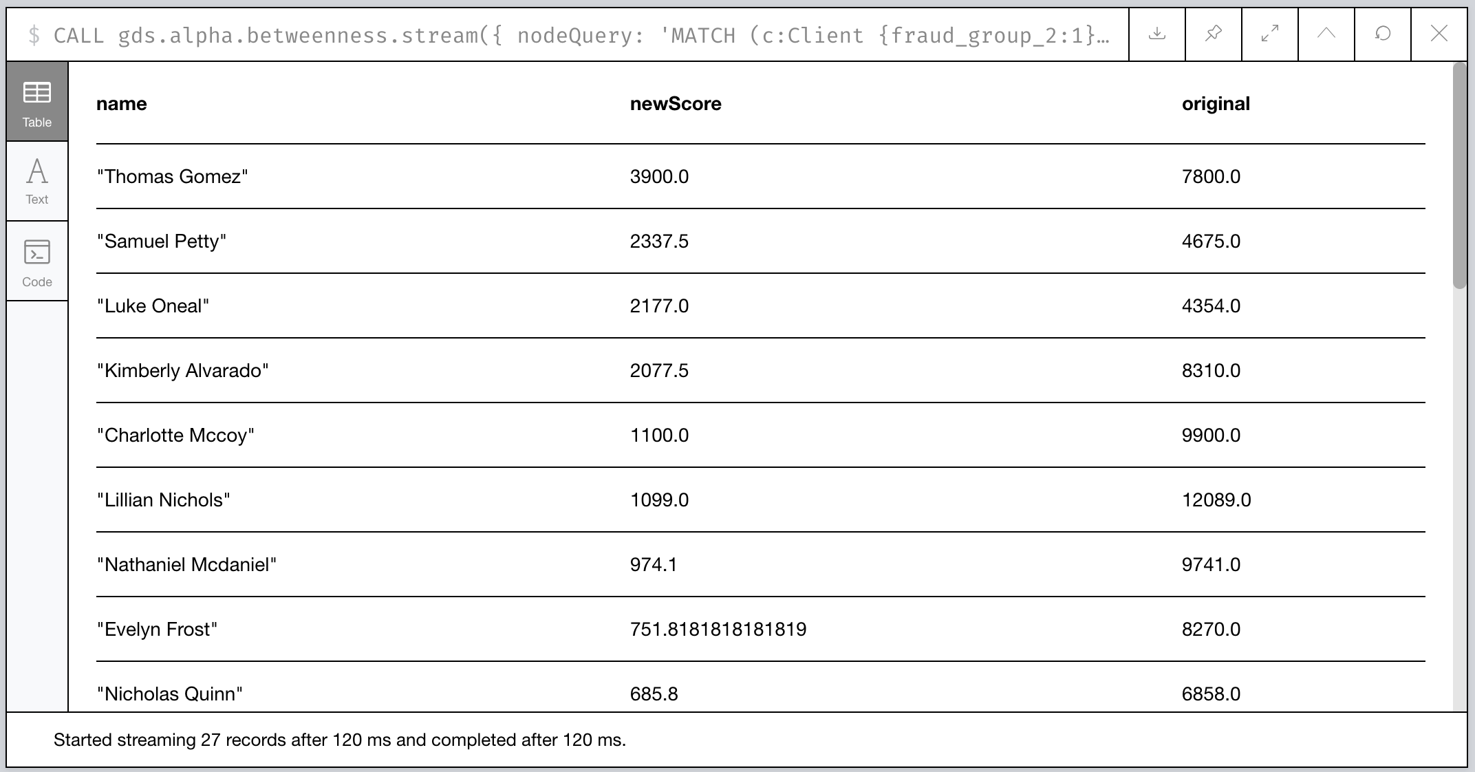
Figure 17: Our bespoke Betweenness Scoring
In Summary: What Did We Find?
To summarize, we used the Graph Data Science library to perform some critical steps in our analysis of our financial transaction data:
- We culled the universe down to potential First Party Fraudsters using Weakly Connected Components (WCC).
- We then isolated the largest groups to target our investigation.
- We expanded our search using the power of Cypher, finding out that the groups we identified looked very different than they first appeared!
- We re-ran WCC and retagged our suspects.
- We algorithmically found a way to identify linchpins in our largest potential fraud network using a combination of Betweenness Centrality and some old fashioned intuition!
Our take-away: look into three particularly shady characters!
🎓 Learning More
Make sure to check out some other great posts about using graphs and graph algorithms to investigate first party fraud.
I recommend Max Demarzi’s previous post and newly revised post on first party fraud for similar look at using algorithms:
- Part 1 in which he uses the previous “Graph Algorithms” library to identify fraud rings
- Part 2 in which he revises it using the newer “Graph Data Science” library we used in this post.
As well as a recent video overview of using Graphs in AI and Machine Learning from Neo4j’s Data Science and AI product managers.
Next Time: Investigating Fraudulent Charges
In the next post in this PaySim series, we’ll look at investigating fraudulent charges and finding potential sources of things like account theft through card skimming. Stay tuned!
👣 Footnotes
-
PaySim (original and my 2.1 version) both have a max transaction limit as well, so the highest possible value is capped. ↩︎
-
But, Dave, doesn’t Neo4j already try to keep the database in memory? Yes, but in this case, the graph algorithms library creates an even more optimized version of the data to speed up application of the algorithms. Check out the docs on the “project graph model”. ↩︎
-
This is what’s called a native projection in GDS-speak. ↩︎
-
See docs on the Cypher projection support in the Ne4j Graph Algorithms documentation. ↩︎
-
For use cases as to when to use Betweenness Centrality, check out the use-cases section of the official documentation. ↩︎